This document (and my interpretation of pulsar astronomy as a whole) is heavily influenced by the layout and workings of the following two books:

A. Lyne , F. Graham-Smith F. Pulsar Astronomy. 4th ed. Cambridge University Press; 2012.
D. R. Lorimer, M. Kramer. Handbook of Pulsar Astronomy. Cambridge: Cambridge University Press, 2005.

I highly recommend the both of them. The former, Pulsar Astronomy, is my personal favourite of the two, and delves better into the theory aspect of neutron stars. The latter, Handbook of Pulsar Astronomy, talks a lot more about instrumentation and methodology, which is very useful for the experiment. Both are “available” in the library, though your mileage may vary.

So you’ve been selected for the Crab Pulsar lab. I’ve decided to write my own pseudo-lab-script, which can be read alongside the real lab script, providing some personal insight on what I found useful on a rather involved but very interesting experiment. A pdf of my own lab book from doing this experiment is also available here.

Neutron Stars and Pulsars

A neutron star is of the most extreme object in the universe. They are the penultimate stage of life for the most massive stars following a type II (core collapse) supernovae. Their gravity is so immense that it overcomes all but the pressure provided by the nuclei of what once was their many different constituent atoms. It becomes energetically favourable under the pressure for nearly all protons to undergo electron capture and become neutrons (you can see where this is going). At this density, the gravity is too strong for any of the neutrons to form bound states with one another, resulting in the main component of a these stars to be fluid neutrons. Hence, the neutron star is born. Should a neutron star be too massive (more specifically, if it exceeds the TOV mass limit), the power of gravity wins out over even the neutron pressure; the star collapses further, into a singularity, giving us our black holes.

Stars, prior to collapse, have some amount of angular momentum. Like every demonstration of angular momentum you’ve seen: if you get smaller, you spin faster. The same holds true for a neutron star. Stars with huge radii of order millions of kilometres are compacted to the size of a city ($\sim20\text{km}$) in a supernova. So it’s safe to say they speed up a considerable amount.

Pulsars are highly magnetised, rapidly spinning neutron stars. We’ve discussed why they spin so fast, but their magnetic field is a little more complicated and beyond the scope of this blog post and lab experiment (we don’t really know). The Crab pulsar is one such star, named due to its location: in the middle of the crab nebulae. It’s one of the most luminous and interesting pulsars we know about, and as a result is observed as often as twice per day. I imagine one of the reasons (if not the main reason) the undergraduates at UoM are allowed to use the 42ft telescope for the Crab Lab is because that’s what the big expensive piece of equipment would be looking at anyway.

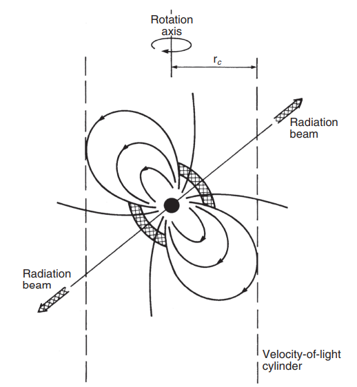
Credit: A. Lyne , F. Graham-Smith F. Pulsar Astronomy. 4th ed. Cambridge University Press; 2012.

They emit lighthouse-like pulses in the radio spectrum as a result of the poles in their magnetic field being misaligned with their rotational axis. These beams alone are very weak, and so there is some amount of finesse required to retrieve information good enough to draw conclusions about a pulsar. Timing pulsars, and understanding why they emit light in the way that they do is important for us to understand the corresponding mechanisms. Due to the extreme conditions within and around a pulsar, understanding the mechanisms can then help us to develop new areas of physics at these extremities where our current model breaks down.

The Lab Script

Let’s take a step back for a second and look back towards the lab script. For us, this experiment could be broken down into three main components:

Dispersion measures of known pulsars (1-2 weeks).
Periodicity of unknown pulsars (1-2 weeks).
Precise timing of The Crab pulsar (2-3 weeks). The times I’ve put in brackets are rough estimates of how long it took myself and my lab partner to perform this, but it is in no way a solid guideline. As you have done a 3rd year lab report by now, you are familiar with the reduced page limit. As such, it makes the most sense to pick only one of these three parts of the experiment to write your lab report on, and I recommend the last.

Radio Astronomy

Basic Radiometer System

There’s some important concepts we need from radio astronomy, before we can do much else. The first we will tackle is as follows: “Why do we need a dish”. The answer is obviously to collect more light. We can put this into numbers using “gain”. We must first understand directivity, a measure of how much of the sky you are looking at:

\[D = \frac{4\pi}{\Omega_A}.\]

Where $\Omega_A$ is the solid angle of the sky which your beam covers. It can be seen that this is simply the inverse of the fraction of sky which the telescope beam covers.

Gain, different from the value given in the exam script, and denoted as such here as $G’$ to reduce confusion, is given by the equation $G’=D\eta$.

\[G' = \eta D = \eta \frac{4\pi}{\Omega_A}\]

Where $\eta$ is the efficiency of the antenna, which often takes on values in the realms of 0.5-0.7. There are plenty of reasons that an antenna dish may not be perfect, such as blockages to the receiver or impurities on the surface, but most important to note is that the efficiency is often purposefully reduced, particularly at the edges of the dish (known as tapering) to reduce the effects of spill-over noise, coming from various radio sources on earth through a feature of the beam known as sidelobes.

The concept of gain is easiest to think of this in terms of an emitter, rather than a receiver. A system emitting isotropically will follow the inverse square law, reducing with distance from the source, such as a star. Now, if you emitted the same amount of energy using an antenna, the flux at the same distance would be multiplied by the gain.

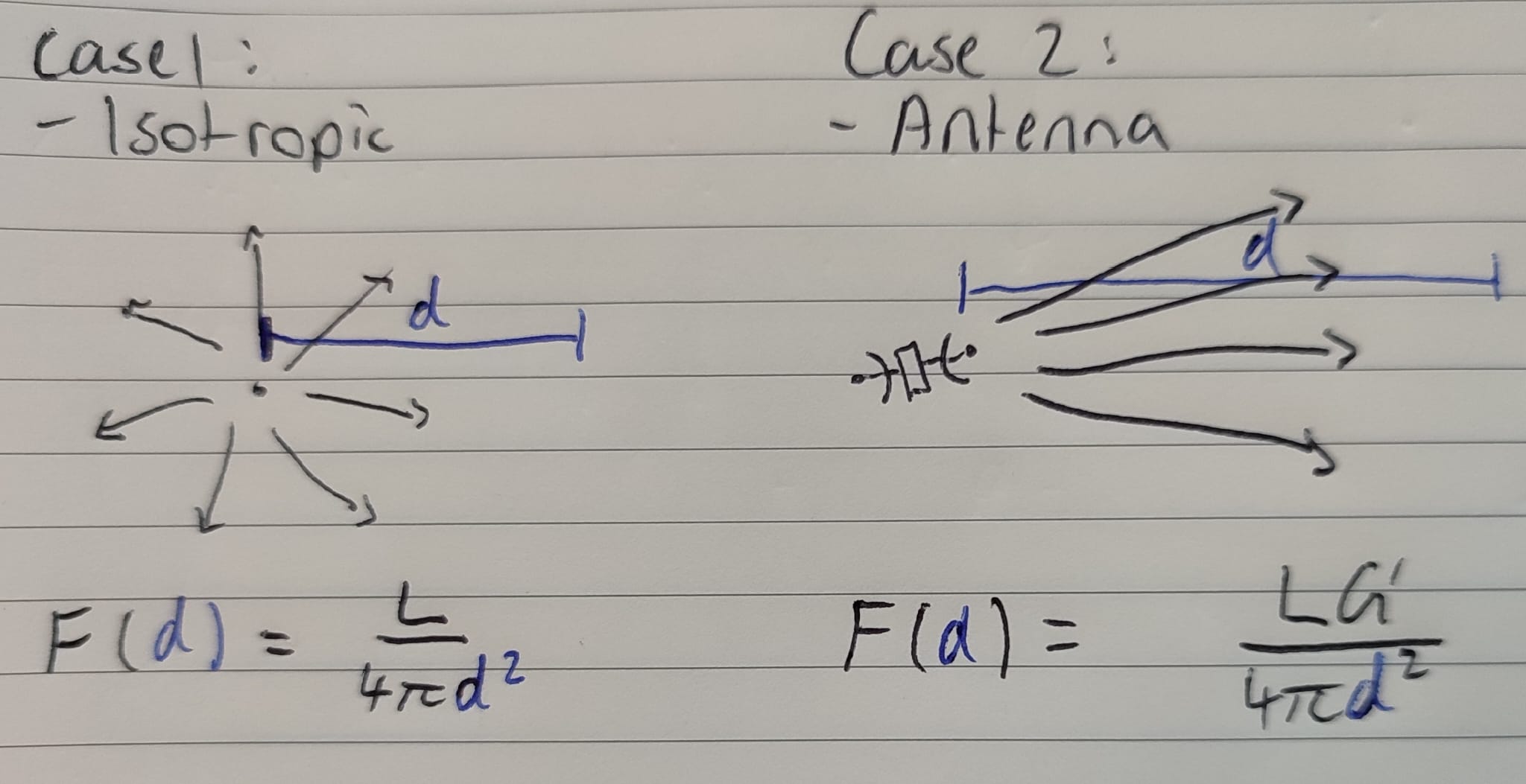
Credit: Me!

Interestingly, the lab script defines gain differently to how I have learned it. It is given as

\[G=\frac{\eta A}{2k_B} = \frac{A_e}{2k_B}\]

where it appears to, instead of being a factor by which we can multiply the flux, is a factor by which we can multiply the increase in temperature. Temperatures and fluxes in radio astronomy are often used as analogues to one-another. A bright source of a certain temperature will cause an increase in temperature of a receiver. Similarly, a receiver at room temperature (or some other temperature) will produce its own radiation at that temperature, creating noise. This is the main reason why radio telescopes are cryogenically cooled, as to avoid this noise.

We still need more tools to derive the equation provided in the lab script, another is the Antenna Theorem. Suppose we put an antenna in a blackbody cavity: an isolated box which no light can escape.

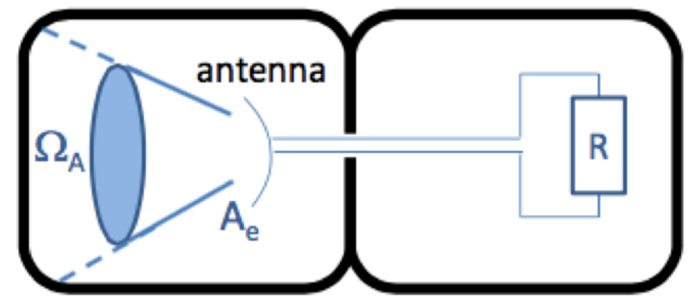
Credit: Radio Astronomy PHYS40591 Slides, Patrick Weltevrede. (Though it is unclear in the slides if this image is from some textbook.)

After some time, this whole system will be in thermodynamic equilibrium. The part of the cavity which the beam can see (i.e. subtends solid angle $\Omega_A$), radiates at its blackbody temperature,

\[B_\nu=\frac{2k_BT}{\lambda^2} \; \text{Wm}^{-2}\text{Hz}^{-1}\text{sr}^{-1},\]

where we have taken the Rayleigh-Jeans limit. The power then collected by the receiver is given by,

\[P_{\text{rec}}=\frac{k_BT}{\lambda^2} A_e \Omega_A \; \text{W}\text{Hz}^{-1}.\]

We have multiplied by the effective area of the antenna, $A_e=\eta A$, and the solid angle of the beam, $\Omega_A$. Additionally, we have lost a factor of two as the antenna can only collect power from a single polarisation. In thermodynamic equilibrium, the receiver has matched the load resistor, shown on the right at temperature $T$, which produces transferrable power $k_BT$ (per unit bandwidth). We can set this equal to our previous expression to obtain the “antenna theorem”:

\[P_\text{rec}=\frac{k_BT}{\lambda^2}A_e\Omega_A=k_BT\] \[A_e\Omega_A= \lambda^2\]

Continuing, we can easily come to the value of $G$ in the lab script with a couple of simple steps following that the antenna theorem must be true. This time, $P_\text{rec}=k_B T_\text{src}$ initially for an unresolved point source and so

\[P_{\text{rec}}=k_BT_\text{src} = \frac{A_e S}{2}\]

We therefore rearrange for $T_\text{src}$ and retrieve

\[T_\text{src} = \frac{A_e S}{2 k_B}=GS\]

giving us a measure for the temperature seen by the receiver as a result of a source of flux density, $S$. By inspection, we can extract $G=A_e/2k_B$ as an analogue to the sensitivity of the dish, and its units are in $\text{K}\text{Jy}^{-1}$

Now it feels as though we are getting somewhere, but we must now talk about statistics. Up until now I have mentioned several sources of ‘noise’ on our receiver system. More of these are mentioned in the lab script and are often quoted as temperature values, and their sum makes up the system temperature

\[\begin{align} T_\text{sys} &=T_\text{source} + T_\text{CMB}+ T_\text{sky} + T_\text{spillover} + T_\text{receiver} + T_\text{atmospheric} +T_\text{attenuation} \\&\approx100\text{K} +3\text{K}+(0.1-3)\text{K} +10\text{K} +(0.1-3)\text{K} +1 \,\text{K} +2\text{K} \end{align}\]

I’ve also provided typical values. Each term is described below:

$T_\text{source}$: What we wish to measure. Flux from the source
$T_\text{CMB}$: Noise contribution from the cosmic microwave background
$T_\text{sky}$: Noise contribution from the sky around the source, such as background galaxies. This depends on frequency and the numbers provided are for 30-1.4$\text{GHz}$, so for 610$\text{MHz}$ I imagine $T_\text{sky}$ sits somewhere a little larger.
$T_\text{spillover}$: Noise contribution from other radio sources (near) perpendicular to the observation direction, detected via the sidelobes.
$T_\text{receiver}$: Noise contribution from the blackbody radiation in the physical receiver system. I have listed it as being between 3K and 28K depending on if the system is cryogenically cooled and depending on the frequency of observation or otherwise. Ask your supervisors if the 42ft is cooled and if so to what extent, because I can’t find any resources online.
$T_\text{atmospheric}$: Noise contribution from the atmosphere. Similarly, this depends on observation frequency, temperature of the atmosphere and height above sea level.
$T_\text{attenuation}$: Noise contribution as the signal travels down the physical cable from the receiver to the amplifier.

It may be the case that some of the sources above are absorbed together in the numbers provided in the lab script.

In an observation of the sky, each of these noise sources will fluctuate around their actual values. As such, to retrieve any useful data we must average out the fluctuations. For some averaging time $\tau_\text{avg}$, the number of coherence times, $\tau_\text{coh}$ (i.e. the time over which the noise is considered to be not varying) is given by

\[N_\text{coh} = \frac{\tau_\text{avg}}{\tau_\text{coh}} = \tau_\text{avg} \; \Delta\nu\]

where we have introduced the relation that the bandwidth, $\Delta \nu$, sometimes referred to $B$ is the inverse of the coherence time. To be able to digitally reconstruct the data, we must sample at least twice per coherence time, this is known as the Shannon-Nyquist theorem and has many applications in data sampling for a multitude of areas of physics and computing. Therefore our number of required samples is

\[N_\text{samp} = 2\tau\Delta\nu\]

where I have dropped the subscript on $\tau_\text{avg}$ in favour of simplicity.

In the final piece of the puzzle we look towards central limit theorem: The sum of any large sample of independent random variables will exhibit a Gaussian distribution. Our variations on received power are not gaussian, but if we average over a long enough time (enough samples) then we should retrieve a gaussian distribution. What is useful about applying CLT is that we know our averaged deviation, $\sigma$ will follow $\sigma_T = \sqrt 2 T_\text{sys}$. The error on the mean for a large sample in CLT is given by

\[\sigma_\mu = \frac{\sigma}{\sqrt{N_\text{samp}}}\]

which we can then introduce our equations for $\sigma_T$ and $N_\text{samp}$.

\[\begin{align} \sigma_\mu & = \frac{\sqrt 2 \; T_\text{sys}}{\sqrt{2 \tau\Delta \nu}} = \frac{T_\text{sys}}{\sqrt{\tau \Delta\nu}}=\Delta T_\text{rms} \end{align}\]

which is the radiometer equation. I’ve introduced the $\Delta T_\text{rms}$ notation, which is the average size of the fluctuations, analogue to the error on the mean of the CLT sample.

You’ll notice this is very similar to the equation given in the lab script. It describes how observation bandwidth, observation time and system temperature all influence the random statistics on measurable readings. The “temperature” of the source needs to exceed this value, $\Delta T_\text{rms}$. Intuitively, this makes sense. Your receiver system needs to see have the signal appear more significantly than the average size of the fluctuations.

We still have the issue that the lab script equation is different from the one we have derived, so to finish off lets create the experiment from the script. $S_\text{SEFD}$ a slightly different analogue to $\Delta T_\text{rms}$ which allows us to incorporate our gain, $G$ from earlier. If you recall gain, $G$, as given by the lab script, was a good representation of the sensitivity of an antenna, we can directly divide our equation in $\Delta T_\text{rms}$ by the gain to find ourselves a similar equation in flux density terms instead.

\[S_\text{SEFD} = \frac{T_\text{sys}}{G\sqrt{\tau \, \Delta\nu}}\]

where $S_\text{SEFD}$ is the source equivalent flux density, or more simply, the flux density required of a source to be resolvable for a given bandwidth and integration time. If you propagate through this working from the Antenna theorem assuming that the number of polarisations your telescope can see is $n_p$, you can also introduce that factor to the above equations, but this lab script is the only place where I have seen it not to be taken right away that $n_p = 1$.

That’s all for now! Hopefully in the (long) time it has taken me to get started with finding the motivation to write up some of this, you have made some solid progress on the required aspects of the experiment. Part II will detail pulsars more specifically, and some of the initial timing and signal processing required to find first results about the Crab pulsar.